VLOOKUP is an Excel function to lookup and retrieve data from a specific column in a table. It supports approximate and exact matching, and wild cards (* ?) for partial matching. The “V” stands for “vertical”. It is an extremely useful function and here is how you can use it.
Syntax
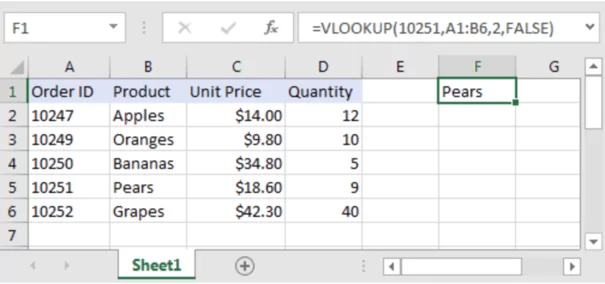
VLOOKUP (lookup_value, table_array, col_index_num, [range_lookup])
Arguments
- lookup_value – The value to look for in the first column of a table.
- table_array – The table from which to retrieve a value.
- col_index_num – The column in the table from which to retrieve a value.
- range_lookup – [optional] TRUE = approximate match (default). FALSE = exact match.
Applies To: Excel 2016, Excel 2013, Excel 2010, Excel 2007, Excel 2016 for Mac,Excel for Mac 2011, Excel Online, Excel for iPad, Excel for iPhone, Excel for Android tablets, Excel for Android phones, Excel Mobile, Excel Starter 2010.
What you’ll need to build the VLOOKUP syntax:
-
The value you want to look up, also called the lookup value.
-
The range where the lookup value is located. Remember that the lookup value should always be in the first column in the range for VLOOKUP to work correctly. For example, if your lookup value is in cell C2 then your range should start with C.
-
The column number in the range that contains the return value. For example, if you specify B2: D11 as the range, you should count B as the first column, C as the second, and so on.
-
Optionally, you can specify TRUE if you want an approximate match or FALSE if you want an exact match of the return value. If you don’t specify anything, the default value will always be TRUE or approximate match.
Now put all of the above together as follows:
=VLOOKUP(lookup value, range containing the lookup value, the column number in the range containing the return value, optionally specify TRUE for approximate match or FALSE for an exact match).
Example
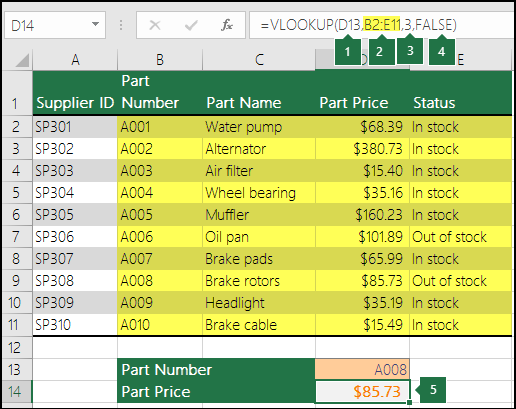
The following picture shows how you’d set up your VLOOKUP to return the price of Brake rotors, which is 85.73.
-
D13 is lookup_value, or the value you want to look up.
-
B2 to E11 (highlighted in yellow in the table) is table_array, or the range where the lookup value is located.
-
3 is col_index_num, or the column number in table_array that contains the return value. In this example, the third column in the table array is Part Price, so the formula output will be a value from the Part Price column.
-
FALSE is range_lookup, so the return value will be an exact match.
-
Output of the VLOOKUP formula is 85.73, the price of Brake rotors.
Sources: Office Support